install.packages("tidyverse")Differential Expression and the Mouse Gut-Brain Axis
This module provides data for an independent project exploring differential expression in RNA-seq data.
This activity will walk through differential expression analysis and use bioinformatics tools (R) to understand how gut bacteria can influence the expression of genes in the brain (the gut-brain axis). You will work with real data from a mouse RNA-seq experiment.
Background
Autism spectrum disorder (ASD) is a neurological disorder that affects behavioral and social interactions, among other things. Although ASD can be diagnosed at any age, it’s considered a neurodevelopmental disorder because symptoms usually show up within the first two years of life. Individuals diagnosed with ASD can experience a wide range of symptoms, including differences in social behaviors and communication styles, as well as intellectual disabilities and physical issues like sensory sensitivities or gastrointestinal problems.
The data for this activity includes gene expression data from two different brain regions (striatum and prefrontal cortex) in mice. Mice in this experiment received fecal transplants. Some mice received transplants from humans who have been diagnosed with ASD, while other mice received transplants from humans who did not have any diagnosis (control). This allowed researchers to control the composition of the gut microbiome in each mouse. Researchers then bred the mice and looked for differences in gene expression in the brains of the offspring.
The striatum is part of the brain involved in motor control and cognitive tasks like reward processing, decision-making, and social interactions (often called executive functions). It lies deep within the center of the brain and is composed of both gray matter (which can be thought of as the “processing” part of brain tissue) and white matter (which is the brain structure involved in transporting messages); the combination of the gray and white matter give this region of the brain a striped appearance, resulting in the name “striatum”. The striatum is involved in both reflexive movement - that is, involuntary movement that happens as an immediate response to a stimulus - and slower, planned movement like walking. In Parkinson’s disease, some patients experience degeneration of parts of the striatum, resulting in spastic, uncontrollable movement.
The prefrontal cortex is the part of the brain that is primarily in charge of decision making, reasoning, personality, maintaining social appropriateness, and other complex behaviors that fall under the umbrella of executive functions. This can include planning, self-control, and working towards long-term goals. The prefrontal cortex is located in the very front of the brain, just behind your forehead. One of the most famous brain injury patients was Phineas Gage, a railroad worker who survived an iron rod through his forehead. His prefrontal cortex was destroyed in this accident, and doctors noted huge behavioral and personality changes. You can read more about his case here.
The original study
The original study, Human Gut Microbiota from Autism Spectrum Disorder Induces Behavioral Deficits in Mice, was published in 2019. Gut microbiota are known to be different between individuals with ASD and individuals who are considered typically-developing. Additionally, some individuals with ASD also experience gastrointestinal symptoms, and their gut microbiota show the greatest difference when compared to the gut microbiota of typically-developing individuals. Some researchers have proposed that gut bacteria can influence some of the symptoms of ASD. The relationship between the intestinal microbiome and the development and function of the human brain is known as the gut-brain axis.
In this study, researchers explored whether they could induce ASD-like behaviors in mice by changing their gut microbiome. They transplanted stool from either humans with ASD or controls into germ-free mice and discovered that colonization with gut microbiota was enough to induce ASD-like behaviors in the mice. They also let the mice breed and collected gene expression data from the brains of their offspring to explore whether changing the gut microbiota could result in changed gene expression. In particular, they discovered that the offspring of mice who received stool from ASD donors showed different gene splicing and expression profiles of certain ASD-relevant genes.
Note
It is important to note that researchers are not suggesting that ASD is entirely induced by gut bacteria. There is a strong genetic component to ASD. Scientists have known for years that there are both genetic and environmental components to the development or severity of some ASD symptoms. This research explores one possible environmental component.
You can read the original research paper here.
The mouse as a model organism
The mouse is the most commonly-used model organism in laboratory work. In fact, mice and rats make up 95% of the lab animal population, and more than 80% of the research that has been awarded the Nobel Prize for Medicine was done at least in part with mouse models (https://www.cshl.edu/of-mice-and-model-organisms/, https://fbresearch.org/medical-advances/nobel-prizes).
So what makes mice such good model organisms for biomedical research? Well, first, they’re economical and relatively easy to keep. Since mice are small, they don’t require a huge amount of space or food. They also have fast reproductive cycles, so researchers can study multiple generations within only a few years. Most importantly, though, mice and humans are both mammals and have about 85% of their protein-coding genome in common. As a result, mouse physiology is quite similar to human physiology. The mouse circulatory, reproductive, digestive, hormonal, and nervous systems are frequently used as models to study how humans grow, age, and develop chronic diseases. They are particularly important model organisms for cancer research and neuroscience.
You can find additional information about how the mouse is used in research here!
Analysis
Before starting this activity, you should have completed the miniCURE activities and identified genes of interest for your individual project. Remember, the basic steps of your analysis are:
Examine expression of your gene of interest expressed in this dataset.
Explore whether your gene of interest is differentially expressed between the experimental groups.
Characterize the genes that are differentially expressed between the experimental groups based on their molecular activity.
Below, we’ve included a cheatsheet of some of the analysis steps you might want to do and the R code that helps you do it.
Start Posit Cloud
In the next steps, we will explore the data from the publication described above.
We will use Posit Cloud for this activity. Go to https://posit.cloud/plans/free and follow the steps to sign up. You can also Log In using the button on the top right if you have used Posit Cloud in the past.
TODO: Add figure
Once logged in, select “New Project” and “New RStudio Project”. It will take a few seconds to deploy and load.
TODO: Add figure
Rename your project “Differential Expression Mouse GutBrain” by clicking on “Untitled Project”.
TODO: Add figure
Package Install and Load
We will need to install the tidyverse package for this activity.
Type the following into your console and press return to run the code. You will see a lot of red text, but usually that’s a good thing!
TODO: Add figure
Next, we will load the package so it’s ready to use:
library(tidyverse)TODO: Add figure
What are R Packages?
Packages are collections of R code, data, and documentation that extend the base functionality of R. Think of them like “expansion packs” on top of your basic R software.
Packages are developed by the R community and made available through repositories like CRAN (Comprehensive R Archive Network), Bioconductor, and GitHub. They are especially useful if you want to do a specialized kind of analysis, such as genomic analysis!
We use the library command to load and attach packages to the R environment. This means links the package you downloaded to your current session of R.
The “tidyverse” package that you loaded is useful for loading, wrangling, and exploring data.
Loading the data
You have the option to look at gene expression in control vs ASD mice, as well as gene expression in both striatum and prefrontal cortex. All the mice were male and sacrificed at the same age (45 days).
Additionally, you can look at gene expression in striatum vs prefrontal cortex in only ASD mice or only control mice. Likewise, you also have the option of looking at gene expression in ASD and control mice, focusing only on striatum or only on prefrontal cortex.
Let’s say you want to open the dataset that compares gene expression between ASD and control mice in both brain regions and call it asd_vs_c. We will do this using read_csv. Copy and paste this command into your console:
asd_vs_c <- read_csv("https://genomicseducation.org/data/mouse_gutbrain_de_autismVcontrol.csv")Rows: 55421 Columns: 7
── Column specification ────────────────────────────────────────────────────────
Delimiter: ","
chr (1): gene
dbl (6): baseMean, log2FoldChange, lfcSE, stat, pvalue, padj
ℹ Use `spec()` to retrieve the full column specification for this data.
ℹ Specify the column types or set `show_col_types = FALSE` to quiet this message.Here are the URLs for all the possible comparisons you can examine with this dataset:
Comparing gene expression between ASD and control mice
Both brain regions: https://genomicseducation.org/data/mouse_gutbrain_de_autismVcontrol.csv
Prefrontal cortex only: https://genomicseducation.org/data/mouse_gutbrain_de_autismVcontrol_in_prefrontalcortex.csv
Striatum only: https://genomicseducation.org/data/mouse_gutbrain_de_autismVcontrol_in_striatum.csv
Comparing gene expression between prefrontal cortex and striatum
All mice: https://genomicseducation.org/data/mouse_gutbrain_de_tissuetype.csv
Only ASD mice: https://genomicseducation.org/data/mouse_gutbrain_de_tissuetype_in_ASDmice.csv
Only control mice: https://genomicseducation.org/data/mouse_gutbrain_de_tissuetype_in_controlmice.csv
Arranging dataset based on padj
You’re mostly interested in identifying the genes that have been differentially expressed between your two groups (in this case, ASD mouse brains and control mouse brains). You can use the arrange command to sort the results to put the smallest padj values first.
asd_vs_c_sorted <- arrange(asd_vs_c, padj)
head(asd_vs_c_sorted)
# A tibble: 6 × 7
gene baseMean log2FoldChange lfcSE stat pvalue padj
<chr> <dbl> <dbl> <dbl> <dbl> <dbl> <dbl>
1 ENSMUSG00000089657 16.9 -25.5 1.81 -14.1 2.18e-45 7.29e-41
2 ENSMUSG00000083812 14.6 -25.4 1.80 -14.1 3.82e-45 7.29e-41
3 ENSMUSG00000094151 11.2 -25.0 1.79 -14.0 2.97e-44 3.77e-40
4 ENSMUSG00000102414 14.9 -25.4 1.89 -13.4 4.00e-41 3.81e-37
5 ENSMUSG00000074445 11.5 -25.0 1.89 -13.3 3.44e-40 2.62e-36
6 ENSMUSG00000053773 10.6 -24.9 1.99 -12.5 6.66e-36 4.23e-32Creating a gene list
Next, you might want to create a list of all the genes that are differentially expressed between your two groups using the filter command. Make sure to check that your gene list has enough genes on it using head and dim (and that you have a good ratio of “real” positive versus false positive results).
This step requires some thought as to what you want to set as your padj threshold! Remember, you want to make sure you have a minimal number of false positive results, while also still keeping enough genes for future analyses.
asd_vs_c_sig <- filter(asd_vs_c, padj < 0.05)
head(asd_vs_c_sig)
# A tibble: 6 × 7
gene baseMean log2FoldChange lfcSE stat pvalue padj
<chr> <dbl> <dbl> <dbl> <dbl> <dbl> <dbl>
1 ENSMUSG00000089657 16.9 -25.5 1.81 -14.1 2.18e-45 7.29e-41
2 ENSMUSG00000083812 14.6 -25.4 1.80 -14.1 3.82e-45 7.29e-41
3 ENSMUSG00000094151 11.2 -25.0 1.79 -14.0 2.97e-44 3.77e-40
4 ENSMUSG00000102414 14.9 -25.4 1.89 -13.4 4.00e-41 3.81e-37
5 ENSMUSG00000074445 11.5 -25.0 1.89 -13.3 3.44e-40 2.62e-36
6 ENSMUSG00000053773 10.6 -24.9 1.99 -12.5 6.66e-36 4.23e-32dim(asd_vs_c_sig)[1] 10 7Exploring genes of interest with the Mouse Genome Informatics database
TODO: Change this so they look up geneIDs for their genes of interest??
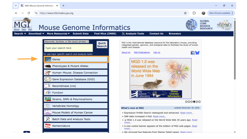
The Mouse Genome Informatics database that tracks mouse genes and expression data. A full introduction to everything available through the MGI can be found here. We’ll reproduce some of it below.
To look up information on a particular gene of interest, choose the “Genes” button.
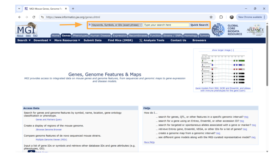
Next, type the gene ID into the “Search” bar up top. We’ll look up “ENSMUSG00000079516”.
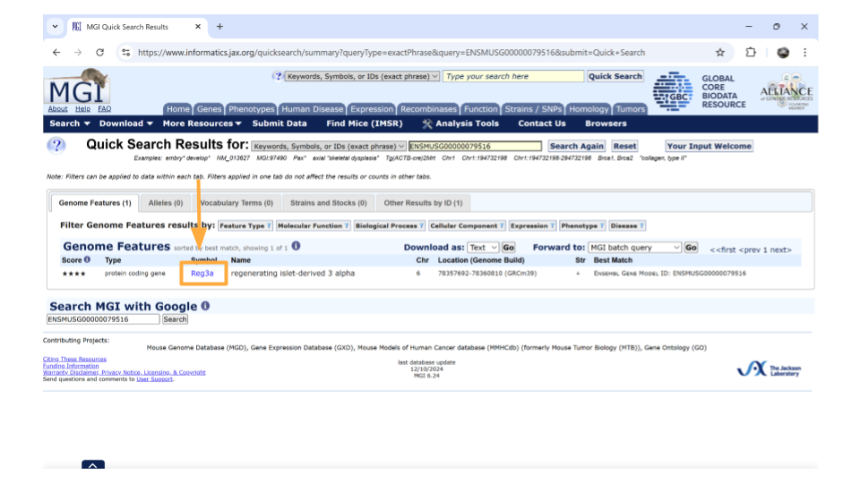
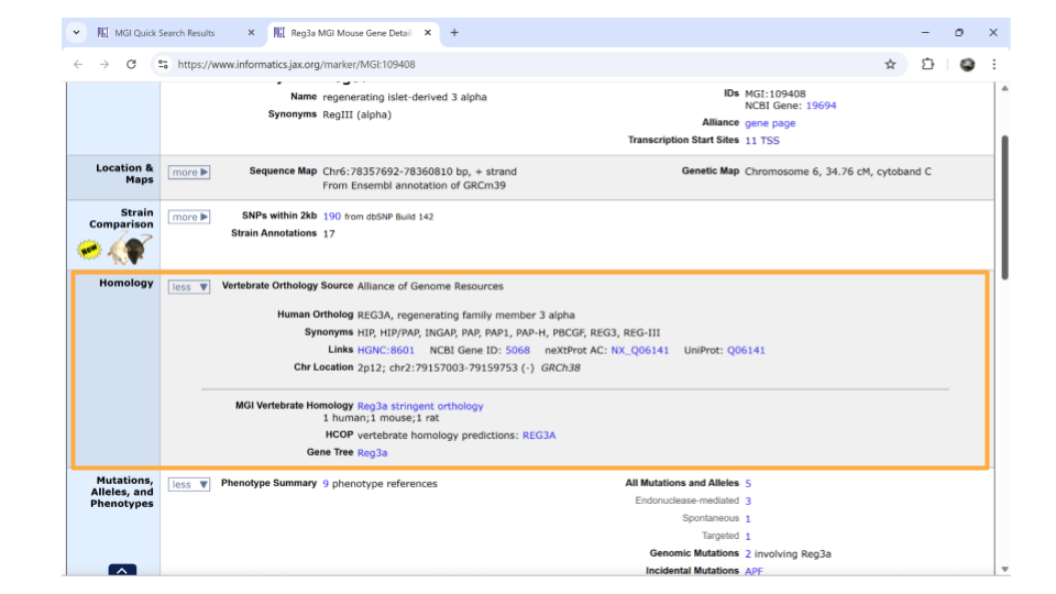
After you type the gene ID into the Search bar and hit enter, you should see a new page with basic information about the gene. Click on the gene symbol (in this example, Reg3a) to get more detailed information.
You might come across some unexpected terms when you search the MGI for your gene ID. In addition to genes, Ensembl gene IDs are also given to “pseudogenes”, “putative genes”, and “lncRNA”.
pseudogene: This is a stretch of DNA that looks like a gene but doesn’t actually code for any protein products. It’s essentially a copy of a gene that contains mutations that prevent translation into a protein product. The mutations can include partial deletions, missing promoters, missing start codons, premature stop codons, frameshift mutations, or missing introns. Any of these are enough to result in a pseudogene.
putative gene: This is a DNA segment that is believed to be a gene, but its function and protein product has not been confirmed. They are frequently identified based on the presence of an Open Reading Frame. Putative genes are not given names until they become confirmed genes.
lncRNA: This stands for “long non-coding RNA”. lncRNA is a type of RNA molecule that is transcribed from DNA but does not code for proteins. These RNA molecules are at least 200-500 nucleotides long and play roles in various biological processes, like gene regulation.
On the new page that you open, details about the gene are organized into familiar categories. Down the left-hand side of the page, you will see sections about the chromosomal location, homology, gene ontology, expression data, and more. Most sections are expanded by default, but you’ll need to expand the “homology” section yourself.
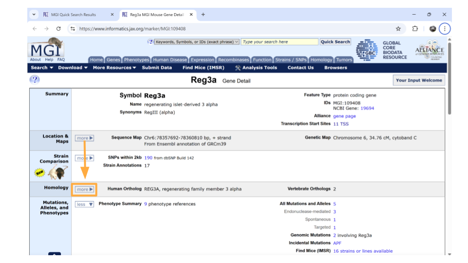
Once this section is expanded, you can find information about possible human homologs to the mouse gene, including alternate names and where the human homolog is located in the human genome.
If you continue scrolling down the page, you can also examine the pathways and processes the gene product is involved in under the “gene ontology” section. Clicking on the blue squares takes you to a page with more information about how that particular gene was assigned to a pathway or molecular process.
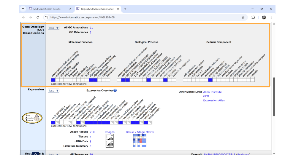
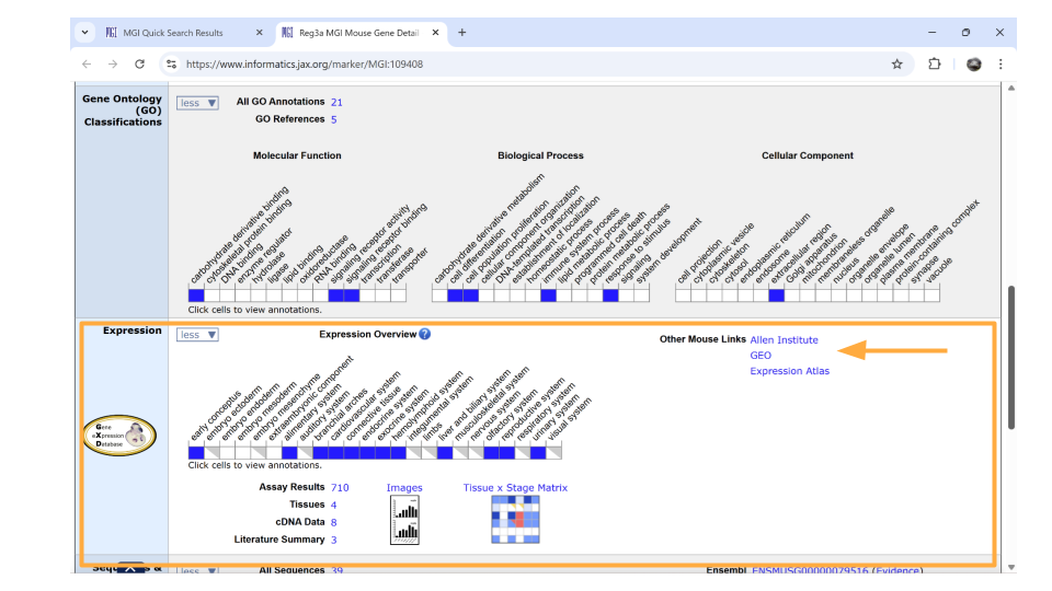
Directly underneath the “ontology” section is information about when the gene is expressed during development. You can learn more information by clicking on the blue squares, or by clicking on the links in the upper right-hand corner. These links will take you to other websites.
Compare differential gene expression across regions
It might be interesting to look at the expression of a gene across all the possible regions. To do this, we will first load the region-specific datasets.
asd_vs_c_prefrontal <- read_csv("https://genomicseducation.org/data/mouse_gutbrain_de_autismVcontrol_in_prefrontalcortex.csv")Rows: 55421 Columns: 7
── Column specification ────────────────────────────────────────────────────────
Delimiter: ","
chr (1): gene
dbl (6): baseMean, log2FoldChange, lfcSE, stat, pvalue, padj
ℹ Use `spec()` to retrieve the full column specification for this data.
ℹ Specify the column types or set `show_col_types = FALSE` to quiet this message.asd_vs_c_striatum <- read_csv("https://genomicseducation.org/data/mouse_gutbrain_de_autismVcontrol_in_striatum.csv")Rows: 55421 Columns: 7
── Column specification ────────────────────────────────────────────────────────
Delimiter: ","
chr (1): gene
dbl (6): baseMean, log2FoldChange, lfcSE, stat, pvalue, padj
ℹ Use `spec()` to retrieve the full column specification for this data.
ℹ Specify the column types or set `show_col_types = FALSE` to quiet this message.Then we’ll filter out the gene in which we’re interested from each object. Let’s take a look at gene ENSMUSG00000079516, which is the reg3a gene we previously looked up on MGI.
reg3a_prefrontal <- filter(asd_vs_c_prefrontal, gene == "ENSMUSG00000079516")

reg3a_striatum <- filter(asd_vs_c_striatum, gene == "ENSMUSG00000079516")
Finally, take a look at the differential expression of reg3a in each region.
In the prefrontal cortex:
reg3a_prefrontal# A tibble: 1 × 7
gene baseMean log2FoldChange lfcSE stat pvalue padj
<chr> <dbl> <dbl> <dbl> <dbl> <dbl> <dbl>
1 ENSMUSG00000079516 10.6 -22.6 2.11 -10.7 7.30e-27 2.63e-23In the striatum:
reg3a_striatum# A tibble: 1 × 7
gene baseMean log2FoldChange lfcSE stat pvalue padj
<chr> <dbl> <dbl> <dbl> <dbl> <dbl> <dbl>
1 ENSMUSG00000079516 0.371 2.27 2.96 0.765 0.444 NAPlotting a single gene across regions
TODO: Figure out the bespoke function `PlotAcrossRegions`
plotAcrossRegions("FBgn0000003")
ENSMUSG00000079516
Running a gene set analysis
You can use the special command runClusterProfiler to figure out the types of processes genes on your gene list are involved in. You can also create a dotplot to visualize your results.
TODO: Verify if `runClusterProfiler` is a bespoke function

asd_vs_c_clusters <- runClusterProfiler(asd_vs_c_sig)

dotplot(asd_vs_c_clusters, showCategory=34, title="a1 vs p1", font.size=10, label_format = 50)
EXTRA UNNEEDED CODE (possibly needed to replace a bespoke function to create a plot across regions): Since we’re working with two separate datasets, let’s add a column to each dataset so we know whether we’re looking at expression data in prefrontal cortex or striatum.
asd_vs_c_prefrontal$region <- "prefrontal_cortex"

asd_vs_c_striatum$region <- "striatum"
If you take a look at both asd_vs_c_prefrontal and asd_vs_c_striatum, you’ll see that the new column has been added on the rightmost side of the data.
head(asd_vs_c_prefrontal)
head(asd_vs_c_striatum)
Next, we’ll combine our two filtered datasets to make one single dataset that only contains expression of the reg3a gene. We’ll combine the datasets with the bind_rows. This command essentially “glues” the two datasets together, one on top of the other.
reg3a <- bind_rows(reg3a_prefrontal, reg3a_striatum)
head(reg3a)